How To Write A Solution Set

Solution Sets of linear systems

What is a solution ready in algebra

A solution set up in algebra refers to the set of values which inputted into a system of equations correctly solve such organization. In other words, these values satisfy the equality of the equations contained in the arrangement nosotros are trying to solve and and so, the list of the corresponding value for each unknown variable in a system conforms the complete set of solutions.

At this indicate, we are no strangers to the idea of solving a set of linear equations, we take done information technology in different ways through past lessons in our Linear Algebra course, such as in the lesson on solving systems of linear equations past graphing or the lesson nearly solving a linear organisation with matrices using Gaussian elimination.

We will continue to use such techniques (generally Gaussian emptying, also known as row reduction) throughout our lesson of today to discover a linear organization solution, but before we continue on to that it is imperative we finally become to know the types of linear systems of equations that we tin find in our problems:

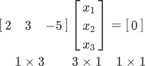
A organization of linear equations is homogeneous if nosotros can write its matrix equation in the form $Ax=0$ . On the other hand, a system of linear equations is nonhomogeneous if nosotros tin write its matrix equation in the grade $Ax=b$ .

We can limited solution sets of linear systems in parametric vector form, simply the blazon of system we accept to work with will make a deviation in the blazon of solutions we can obtain:

• Types of solutions a homogeneous system tin can have in parametric vector form:
• With one gratis variable: $x=tv$
• With 2 free variables: $x=su+tv$
• With n free variables: $x=av_{i}+bv_{2}+...+nvn$


• Types of solutions a nonhomogeneous system can have in a parametric vector class:
• With one free variable: $x=p+tv$
• With 2 gratis variables: $ten=p+su+tv$
• With n costless variables: $ten=p+av_{1}+bv_{2}+...+nv_{north}$

Where 10 represents the column vector containing all of the corresponding unknown variables from the linear system. $u$ , $v$ and $v_{1, ii ... n}$ represent the cavalcade vectors formed by the coefficients of each unknown variable in each equation from the system; while $due south$ , $t$ and $a$ , $b$ , ... , $n$ are the free variables.

For the instance of nonhomogeneous systems you volition have an extra vector coming out in the solutions, this actress vector is what we accept named $p$ higher up.

How to find a solution set of an equation

The bones steps to follow when computing solution sets for a system of linear equations are:

1. Convert the linear system into a matrix equation
2. Rewrite the matrix equation as an augmented matrix
3. Compute the reduced echelon form of the augmented matrix using Gaussian elimination
4. The reduced echelon class of the matrix will provide the values (or expressions) for the unknown variables, use these solutions to write down the parametric vector equation form which will contain the complete ready of solutions for the system.

All of these steps will be explained in particular in the do examples provided in the last section of this lesson. For now, it is important that if you have any doubtfulness on how to work through any of the steps mentioned to a higher place, y'all revisit the next by lessons: representing a linear organization as a matrix, row reduction and echelon forms and matrix equation $Ax=b$ .

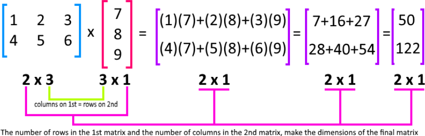
Earlier nosotros continue onto the adjacent section of this lesson, let us have a quick review of something nosotros have been mentioning many times throughout our lessons: matrix multiplication!
Beneath yous tin can find the diagram containing the general rules for matrix multiplication. Y'all must be already familiarized with this diagram since we have included information technology in lessons earlier. The reason why we bring this i up, is that in order to produce matrix equations we will be looking into matrix multiplications (the matrix equations $Ax=0$ and $Ax=b$ are matrix multiplications themselves!), and and then, merely accept the next diagram as a reference for after parts of this lesson where you lot will be working on practise examples.

Equation one: Matrix multiplication

What is a trivial solution in linear algebra

A vector is called trivial if all its coordinates are 0, for example, if it is the zero vector
In Linear Algebra we are not interested in only finding one solution to a organisation of linear equations. We are interested in all possible solutions. In detail, homogeneous systems of equations (see above) are very of import. The important question for a homogeneous arrangement is whether or not there is any non-piddling solution, i. e. whether at that place is any solution other than the trivial one. Sometimes there volition exist, sometimes there wont. Paradoxically, its actually the case where the fiddling solution is the only possible ane that is the nigh important. This situation is described by ane of the most of import words in the whole class.

Find solution set

For this concluding section of our lesson of today, we will be looking for the solutions sets of linear systems. As usual, we volition be using notation of matrices in order to find the corresponding matrix solution set required in each case.

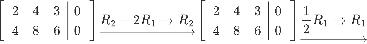
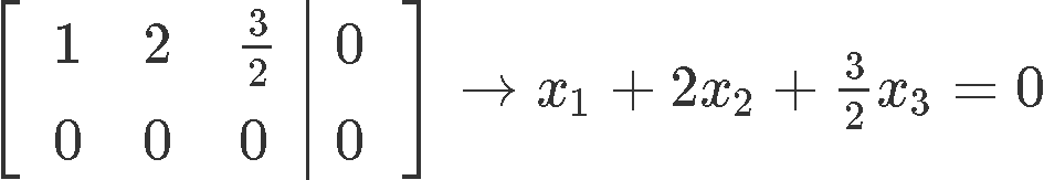
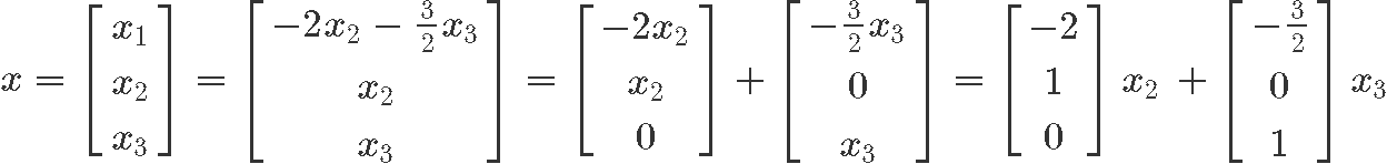
Instance 1

Find the solution set of the homogeneous system in parametric vector class:

Equation two: System of linear equations

Equally we have been doing then for a few lessons at present, nosotros transform this organisation into an augmented matrix and then row reduce information technology until we obtain its reduced echelon form in club to find the final expressions for the variables of the system:

Equation iii: Row reducing the augmented matrix

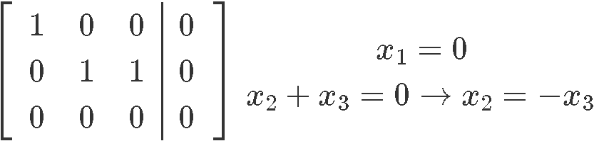
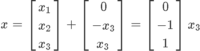
As you can come across from the results above, $x_{3}$ happens to exist a gratuitous variable since in that location is no pivot corresponding to its column in the augmented matrix. And so, the final solution set for system of equations shown in equation 10 is:

Equation 4: Terminal solution set in parametric class

Example ii

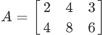
Given matrix $A$ , find the solution ready $Ax=0$ in parametric vector form:

Equation 5: Matrix A

Nosotros write downwardly the matrix equation $Ax=0$ post-obit the rules of matrix multiplication:

Equation 6: Matrix equation Ax=0

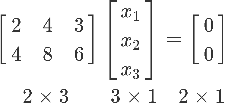
We use this matrix equation to write an augmented matrix which we can solve for the unknown variables equally follows:

Equation 7: Reducing the augmented matrix

By computing the reduced echelon form of the augmented matrix we tin can observe how we are left with no pivots for the second and third column, which means the variables $x_{ii}$ and $x_{3}$ are free variables. And then, we write the solution set of linear equation eight in parametric form every bit shown below:

Equation 8: Last solution set in parametric grade

Example 3

Notice the solution set for the nonhomogeneous system in parametric vector form:

Equation 9: System of linear equations

Writing downwardly the corresponding matrix equation for the linear organisation:

Equation 10: Matrix equation from the system of linear equations

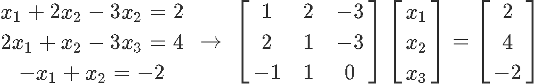
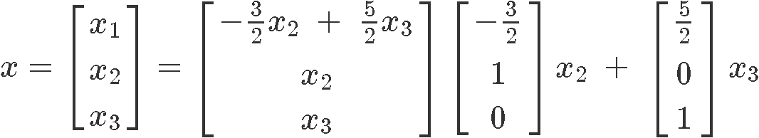
We catechumen this matrix equation into an augmented matrix and row reduce it into we tin obtain the unknown variables expressions:

Equation 11: Row reducing the augmented matrix

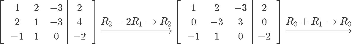
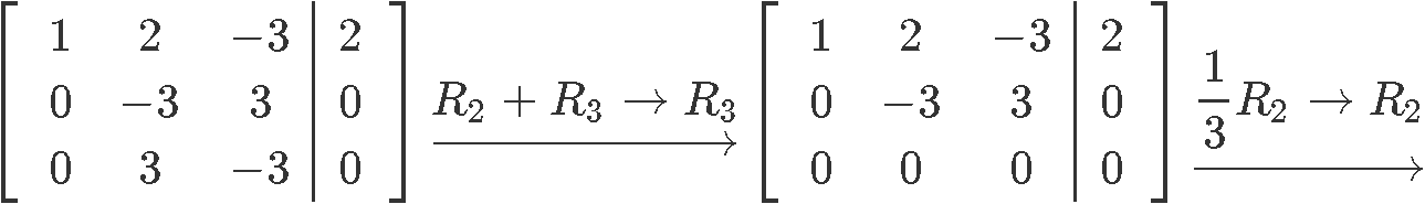
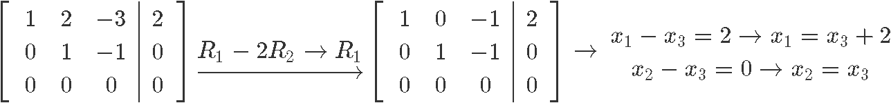
As you can see, the variable $x_{3}$ is a free variable and so the final solution set up for this nonhomogeneous system in parametric grade is:

Equation 12: Final solution prepare

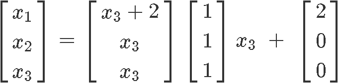
Notice how our final solution set up contains an extra vector without a variable gene. This is ordinarily the case for nonhomogeneous systems equally yous will see in the adjacent examples.

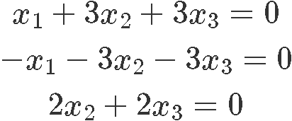
Example 4

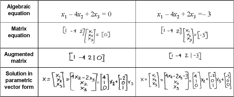
Draw and compare the solution sets for each of the nest two linear equations:

$2x_{i} + 3x_{2} - 5x_{3} = \,$ 0 $\;$ and $\; 2x_{ane} + 3x_{2} - 5x_{iii} = \,$ 4

Equation 13: A homogeneous and a nonhomogeneous linear equation

For this example, each equation happens to accept its own solution set, and thus, we can obtain a matrix equation, then an augmented matrix to finally get in to the parametric vector form of the solution set with each equation.
Since we volition be solving for the solution set of a linear equation at a time, permit the states begin with the homogeneous equation (the one on the left in equation westward). We start past writing down its corresponding matrix equation:

Equation 14: Matrix equation

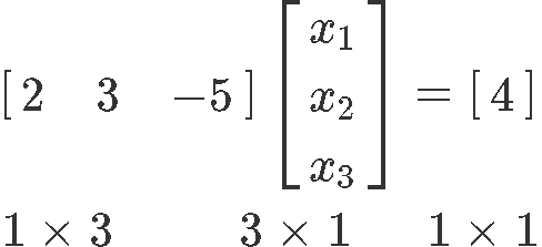
Although making a matrix equation out of a single algebraic equation may seem trouble some, we just take to follow the rules of matrix multiplication shown in equation ____ to construct the equation equally has been shown above. The numbers in the bottom of the equation represent the dimensions of each element in the multiplication: The first factor in the multiplication (the left-about matrix) has one row and three columns, followed by the next factor with three rows and one column. This makes sense since in guild to multiply ii matrices, the first 1 must contain the same number of columns as the second one has rows. And and so, the consequence of such multiplication must ever have the dimensions coming from the number of rows from the first matrix and the number of columns from the second matrix.

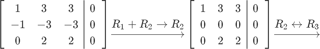
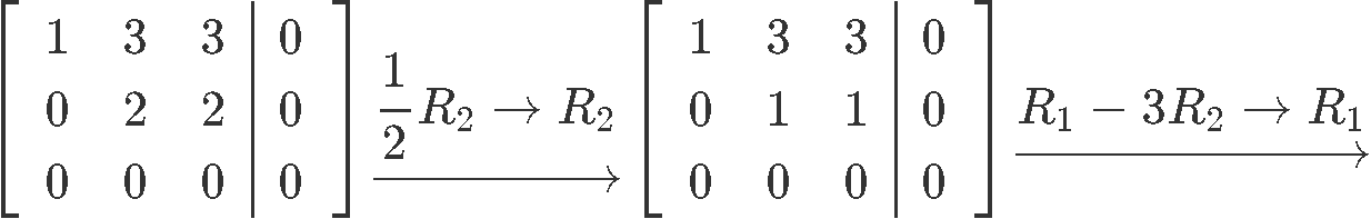
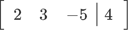
So, the augmented matrix corresponding to the matrix equation above looks like:

Equation 15: Augmented matrix

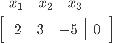
Notice we take written the names of the variables existence represented in each column of the matrix, this, merely every bit the dimensions of the matrices in equation 14, is not needed. We have elected to write these specifications downwards so the computations tin can be shown clearly.
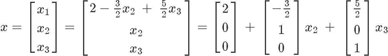
From the augmented matrix we can conclude that the variables $x_{ii}$ and $x_{3}$ are gratis variables. And so, we write down the final solution set for this homogeneous equation:

Equation xvi: Last solution fix for homogeneous equation

Now permit united states of america obtain the linear solution of the nonhomogeneous equation (the correct-near equation from the ready institute in equation w) in parametric vector form. Nosotros start by writing down its respective matrix equation:

Equation 17: Matrix equation

Which will produce the augmented matrix below:

Equation 18: Augmented matrix

And the solution in parametric vector form is:

Equation 19: Concluding solution set for the nonhomogeneous equation

Find that the difference between the two solutions (equations 16 and 19) is just an actress vector resulting from the nonzero value of the nonhomogeneous equation.

Example 5

For this problem we are going to follow the exact same process as we did in the past case to solve the ready of linear equations provided. To facilitate the comparing between the ii results, we accept designed a table in which nosotros accept inputted the computation result of each stride of the procedure:

$x_{ane} - 4x_{2} + 2x_{iii} = \,$ 0 $\;$ and $\; x_{1} - 4x_{2} + 2x_{three} = \,$ -3

Equation twenty: Set up of linear equations provided

Now let u.s.a. go through the entire procedure of the solution set in algebra inside the side by side table:

Tabular array 1: Summary of description and comparison of the process to obtain a solution set from linear equations

Notice that variables $x_{2}$ and $x_{3}$ are free variables. And the difference between the solution of each equation is that the nonhomogeneous equation produces an actress cavalcade vector on its parametric solution.

***

To proceed the practice on solving a gear up of linear equations nosotros recommend y'all to take a look at these algebra notes on solutions and solution sets of linear systems, both links contain some more than examples similar to the ones we accept studied today.

It is the end of this lesson, see you in the next one!

Source: https://www.studypug.com/linear-algebra-help/solution-sets-of-linear-systems

Share this post